Showing posts with label Reference& Lookup Functions. Show all posts

How to use OFFSET Function | Microsoft Excel

October 22, 2018 0
Offset Function

The offset function is working on a reference cell and it will give you a result from the intersection of the column and row.

You should know about offset function if you really want to do fast and precise work on excel.

Syntax of OFFSET Function

=OFFSET(reference,rows,cols,[height],[width])

Arguments of OFFSET Function

Required
reference: Reference is a point from where a counting start for row and columns, it could be a cell or a range.
rows: it is a row number in which you have to find your data. The counting of the row number starting from 0. where a reference cell count as 0
cols: it is a column number in which you have to find your data. Same as the row the counting of the column number starts from 0. where reference cell is count as 0

Optional

height: if you are counting for more that one row then you have to show how much rows participate in the process
width: if you are counting for more that one column then you have to show how much columns participate the processes.

Behavior of OFFSET Function


Here we have to find marks of social studies in the second exam.

we have used a simple formula
=OFFSET(A2,2,3)
Where 
A2 is a reference cell
2 is a row number, the numbering of the row is starting from a reference cell (reference cell will count as 0 after then cell number counted as 1,2,3...). The second row is the Second Exam
3 is a column number, The third column is a Social Studies
so output will be the intersection of the row number and column number which is 55
the value of the second exam in social studies is 55

Usage of OFFSET Function

The usage of the offset function is to find a specific value using row number and column number

Return of OFFSET Function

OFFSET function will return reference value from the intersection of the row and column.

Error values

Error Commands
Description
#VALUE
You have made mistake with reference cell or adjacent cell
#REF
Offset reference of rows and column are over the edge of worksheet

How to Use CHOOSE Function | Microsoft Excel

August 30, 2018 0
how to use choose function

CHOOSE Function is used to get one indexed value from the list of the values. 
For example, there are 7 days Monday, Tuesday, Wednesday, Thursday, Friday, Saturday and Sunday and  the days have arranged in sequence 1 to 7. 1=Monday, 2=Tuesday... and so on
You have to use CHOOSE Function to get the value. If you use 2 number then CHOOSE Function will return the second day(Tuesday) from the list,  If you use 5 number then CHOOSE will return the fifth day(Friday) from the list.

Syntax of CHOOSE Function

=CHOOSE(index_num,value1,[value2]...)

Argument For Choose Function

index_number: it is a number of the index value to return data from the list. Index number should be in between 1 to 254
value1,[value2]...: it can be a list, reference, and any data 

Behavior of CHOOSE Function

how to use choose function
For Example,
You have four month names January, February, March, and April are in a sequence of 1 to 4.
You are using the function 
=CHOOSE(3, C4,C5,C6,C7)
Here 3 is the index number which indicates the value on the 3 rd number must be returned from the list.
For this, the CHOOSE function will return the value located on cell number C6, Which is March.

Return of CHOOSE Function

CHOOSE Function will return the data of the index value from the list

Usage of CHOOSE Function

CHOOSE Function is used to get a single value from the list by giving an index number

Error Values For CHOOSE Function

Error CommandsDescription
 #VALUE
Index number is less than 1 or greater than last value 

More Examples

Example 1 Giving an opinion from 1 to 5 as 1 For Excellent, 2 For Good, 3 For Average, 4 For Poor, 5 For Disgusting.

Here you have five values and five data.
how to use choose function

Values

You have to write five values and data in a column as shown in the figure. here data and values are placed as per above description. 1 For5 Excellent .... 5 For Disgusting

Returns

Choose function will return the opinion as per the numbering from 1 to 5.
CHOOSE function fetches the number in cell E4 and return the value assigned to the reference data which is cell number C5 is AVERAGE.
This is the same for number 1 to 5 where 5 will return Disgusting.
_________________________________________________________________________
How would you like this content to write us in the comment box!
If you face any difficulty in the content feel free to ask!
Thank You.

How to Use MATCH Function | Microsoft Excel

August 22, 2018 0
how to use match function in excel

MATCH function is a lesser known function. Match function will return a position of the specific value given by you from a row and a column.

Syntax of MATCH Function

=MATCH(lookup_value,lookup_array,[match_type])

Arguments For MATCH Function

lookup_value: it is a value which you want to match in lookup_array
lookup_array: it is an array in which lookup_value is search
match_type: value is -1,0 and 1. How lookup_value searched in lookupo_array. the default value is 1

Match Type Description
-1 Describes: Match function finds the smallest value which is greater than or equal to the lookup_value
0 Describes: Match function finds the value which is exactly equal to lookup_value
1 Describes: Match function finds the largest value which is lesser or equal to the lookup_value

Behavior of MATCH Function

how to use match function

Here I want to know the position of March month
So I used the formula
=MATCH("March",B4:B9,)
March:  the value we want to know the position
B4:B9: Range of the data
After using this formula result we get is "3" because March is in the 3rd position in the data

Usage of MATCH Function

To know the position of the given value

Returnof MATCH Function

The position of the value

Note
You can not select more than one column for the data

Error Values of MATCH Function

Error CommandsDescription
#NALookup_value is not available in the range
If you select more than one column or row for a data range

How To Use INDEX Function | Microsoft Excel

August 22, 2018 0
how to use index function in excel

INDEX Function will return you a specific value from the table.

Index function calculates the given row number and column number from the table and returns the intersection value.

Syntax of INDEX Function

=INDEX(array,row_num,[column_num])

Arguments of INDEX Function

array: range of data or a table
row_num: row number from the table which value you want in return
column_num: column number from the table which intersects the row number and returns value

Behavior of INDEX Function

how to use index function in excel

Here you want to see a price for the month of April.
So you have to select a table and apply the formula.

=INDEX(B4: E9,4,3)
Here
B4: E9 is a table
4 is a row number
3 is a column number

This formula will return you the intersection of row and column from the table
The result is "1100"

Usage of INDEX Function

To get a specific value from the specified row and column object from the selected table

Return of INDEX Function

A specific value where a condition is applied

Notes

If there is one row and one column in the table so row number and column number will be optional

Error Values

Error CommandsDescription
#REFMIstake in Row number or Column number
MIstake in syntax
#VALUEIf you use Manual selecting an array you must use CLTR+SHIFT+ENTER for { } bracket otherwise this error appeared
How would you like this content to write us in the comment box!
If you face any difficulty in the content feel free to ask!
Thank You.

How To Use VLOOKUP | Microsoft Excel

February 01, 2018 0
Vlookup

VLOOKUP is most useful function in organizations. It gives you specific detail you want on search of its parameter.

I have created a excel sample sheet to learn.
In sheet1 there is all data of customers (50). Customer’s customer id, ac no, name, scheme code, city, state and country.

Vlookup

We learn how to use VLOOKUP for searching specific value for specific object (customer).

FOR EXAMPLE

If you have customer id of customer and you want to find its mobile no.
you have customer id AX12406 and you find mobile no.
Your source file is sheet1 in which all the data of everyone who is your object (customer).
Your return file is sheet2 which gives you result you need.
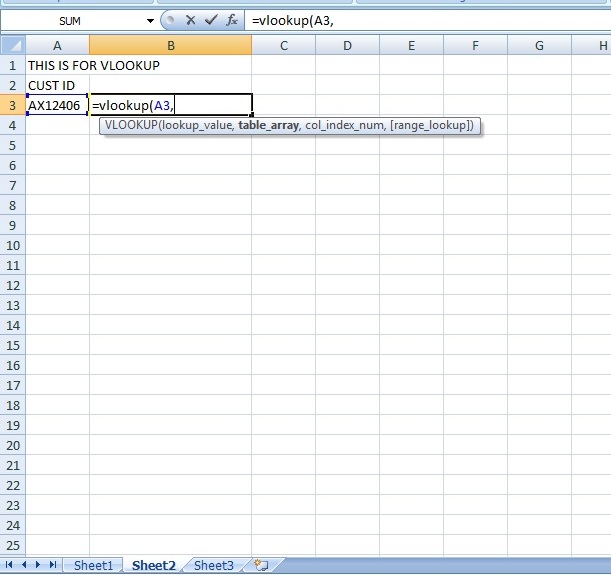
STEP 1: In sheet 2 you have to write customer id AX12406 (Whose mobile no you want)
Vlookup

STEP2: In next cell you have to use function vlookup, enter “=vlookup(“ and select cell where you have entered customer id and place comma(,).
Vlookup

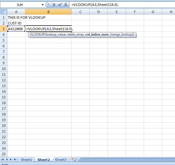
STEP3: Then you have to select range of the date from sheet 1, which data you need must be in range.
Vlookup

STEP4: Back to the sheet 2, first place comma(,).Verify that is must be shee1  in function we use.
Vlookup

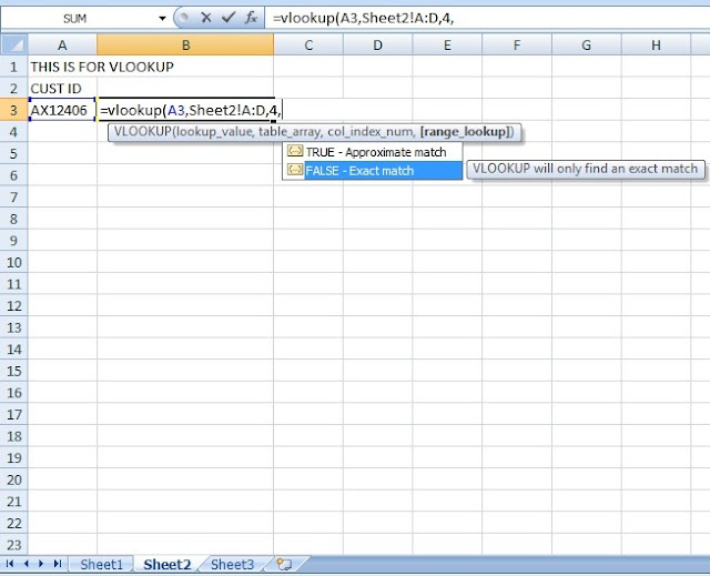
STEP 5: Then write 4, because in the 4th column (of sheet1) we have entered mobile number of our customers.
Vlookup

STEP 6: Then place comma(,). You can see two options.
                1. True-Approximate Match
                2. False-Exact match


We have to select option 2. False Exact match option and then press enter.

Vlookup

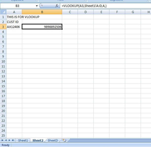
STEP 7:  The result in respected cell


Vlookup

Thanks for reading.
If you have any query, write down in comment box